Steady State Heat Transfer¶

Introduction¶

The module steadystate contains functions that can be used to solve a variety of one dimensional (1D) steady state heat transfer problems related to the following modes of heat transfer:

Conduction
Convection
Radiation

There are four class definitions to model the following geometrical shapes:

Slab (to model rectangular objects)
Cylinder (to model cylindrical objects)
Sphere (to model spherical objects)
CylinderBase (to model flat circular surface)

Each of the above classes implement methods to find:

Heat transfer rate for conduction
Heat transfer rate for convection
Heat transfer rate for radiation
Resistance to conductive heat transfer
Resistance to convective heat transfer
Resistance from fouling

In addition, for ‘Cylinder’ and ‘Sphere’, methods are available to compute their ‘area’ and ‘volume’, while For ‘CylinderBase’, a method is available to compute its ‘area’. No ‘area’ or ‘volume’ methods have been implemented for the class ‘Slab’.

How to use

It is recommended that the module be imported as from pychemengg import steadystate as ss.

The following examples demonstrate how the module steadystate can be used to solve heat transfer problems.

Examples¶

Example 1: Rectangular system `conduction`¶

Example 1. Determine the heat flux q and the heat transfer rate across an iron plate with area A = 0.5 m2 and thickness L =0.02 m (k = 70 W/m °C) when one of its surfaces is maintained at T1 = 60 °C and the other at T2 = 20 °C. Ans: heat rate = 70 kW

# EXAMPLE 1
from pychemengg.heattransfer import steadystate as ss
# Create instance of Slab and call it wall.
wall = ss.Slab(thickness=0.02, area=0.5, thermalconductivity=70)
# Next call on the method of Slab for heat conduction.
# This method needs dT.
# Since the walls are at 60 and 20, dT = 60-20.
# Heatrate can now be computed.
heatrate = wall.heatrateof_cond(dT=60-20)
# Next divide by area of wall to get flux.
# The area can be typed again, but it is stored in the
# attribute 'area' of the instance, so it can be used.
heatflux = heatrate/wall.area
# Result can be printed.
print(f"heatrate = {heatrate} W")
print(f"heatflux = {heatflux} W/m2")

# PRINTED OUTPUT
heatrate = 70000.0 W
heatflux = 140000.0 W/m2

Example 2: Rectangular system `conduction`¶

Example 2. The heat flow rate through a wood board L = 2 cm thick for a temperature difference of ∆T = 25 °C between the two surfaces is 150 W/m2. Calculate the thermal conductivity of the wood. Ans: k = 0.12 W/m °C

# EXAMPLE 2
from pychemengg.heattransfer import steadystate as ss
# Create instance of Slab and call it board.
# Since area is not known, let area  = 1.
# Since thermal conductivity is to be computed, call it 'x'.
# Create a function that can be solved for 'x' as follows.
def func(x):
    board = ss.Slab(thickness=2e-2, area=1, thermalconductivity=x)
    # Heat flux is given, so use it form an equation like so:
    # Compute heat flux = heatrate/area.
    # Since area = 1, heat flux = heat rate.
    flux = board.heatrateof_cond(dT=25)
    # This flux should equal = 150 (given). Thus flux-150 =0.
    # Therefore, the equation to solve becomes:
    equation = flux - 150
    # This equation can then be returned from this function.
    return equation

from scipy.optimize import fsolve
# Typically these import statements are placed at top of code.

# Use fsolve to solve for 'x'
guess_thermalconductivity = 100
# Guess is required to solve, and this is a random value.
# User can change it and the result should be the same.

# Pass function and guess value to fsolve.
solution = fsolve(func, guess_thermalconductivity)
thermalconductivity = solution[0]
# Because output of fsolve is an array, use [0] to get the value.
# Print the result.
print(f"Thermal conductivity = {thermalconductivity} W/mC")

# PRINTED OUTPUT
Thermal conductivity = 0.12 W/mC

Example 3: Rectangular system `convection`¶

Example 3. An electrically heated plate dissipates heat by convection at a rate of q = 8000 W/m2 into the ambient air at Tf = 25 °C. If the surface of the hot plate is at Tw = 125 °C, calculate the heat transfer coefficient for convection between the plate and the air. Ans: h = 80 W/m2 °C

# EXAMPLE 3
from pychemengg.heattransfer import steadystate as ss
# The plate can be modeled as a Slab.
# Since convection is from surface, thickness and thermal conductivity
# are not relevant. These keywords are by default set to 'None'
# and can be ignored. Set area = 1 because it is relevant and
# by setting it to unity the heatrate becomes heatflux.
plate = ss.Slab(area=1)
# Compute heat rate of convection. Two keywords are needed for it,
# heattransfercoefficient and dT. dT = 125-25, but heat transfercoefficient
# need to be determined. Therefore, a function must be setup to solve
# with fsolve.
def func(x):
    flux = plate.heatrateof_conv(heattransfercoefficient=x, dT=125-25)
    # This flux should equal 8000, thus flux-8000=0 is the equation to solve.
    equation = flux-8000
    return equation

from scipy.optimize import fsolve
# Typically these import statements are placed at top of code.
guess_heattransfercoefficient = 1
# Guess is required to solve, and this is a random value.
# User can change it and the result should be the same
solution = fsolve(func, guess_heattransfercoefficient)
heattransfercoefficient = solution[0]
# Because output of fsolve is an array, use [0] to get the value.
print(f"Heat transfer coefficient = {heattransfercoefficient} W/m2C")

# PRINTED OUTPUT
Heat transfer coefficient = 80.0 W/m2C

Example 4: Rectangular system `convection + radiation`¶

Example 4. A small, thin metal plate of area A m2 is kept insulated on one side and exposed to the sun on the other side. The plate absorbs solar energy at a rate of 500 W/m2 and dissipates it by convection into the ambient air at T∞ = 300 K with a convection heat transfer coefficient h = 20 W/m2 °C and by radiation into a surrounding area which may be assumed to be a black body at Tsky = 280 K . The emissivity of the surface is ε = 0.9. Determine the equilibrium temperature of the plate. Ans: 315.4 K

# EXAMPLE 4
from pychemengg.heattransfer import steadystate as ss
# Model the object with Slab.
# Because it is a thin plate, thickness = 0, but thickness is not
# involved in radiation so it can be left = None (default). Area is also not
# known, and since flux is given use area = 1. Thermal conductivity is not
# required because conductive heat transfer is not considered.
plate = ss.Slab(area=1)

# Apply energy balance.
# Energy absorbed = Energy lost by convection + Energy lost by radiation ..(1)
# Convection and radiation involve surface temperature, which is
# the unknown here. Create a function that can be used by fsolve.
# The function will return equation (1).
def func(Ts):
    E_absorbed = 500
    E_conv_loss = plate.heatrateof_conv(heattransfercoefficient=20, dT=Ts-300)
    E_rad_loss = plate.heatrateof_rad(T_infinity=280, T_surface=Ts, emissivity=0.9)
    # NOTE: radiation calculation MUST use absolute temperature.
    # Also note temperature of 300 K is used with convection,
    # and 280 K with radiation.
    equation = E_absorbed - E_conv_loss - E_rad_loss
    return equation

from scipy.optimize import fsolve
# Typically these import statements are placed at top of code.
guess_surfacetemp = 1
# Guess is required to solve, and this is a random value.
# User can change it and the result should be the same.
solution = fsolve(func, guess_surfacetemp)
surfacetemp = solution[0]
# Because output of fsolve is an array, use [0] to get the value.
print(f"Surface temperature of plate = {surfacetemp} K")
# NOTE: Answer is in absolute scale (K in this case)

# PRINTED OUTPUT
Surface temperature of plate = 315.42531589902273 K

Example 5: Rectangular system `composite wall, conduction`¶

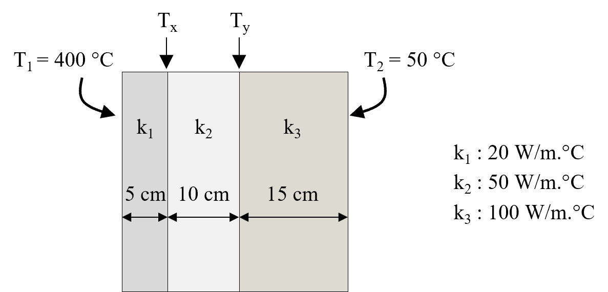
Example 5. A composite wall has three layers with perfect thermal contact as shown below. The outermost surfaces are at T₁ = 400 C and T₂ = 50 C. The thickness of each layer and the respective thermal conductivities (k_i where i = 1,2,3) are also given. Find the heat transfer rate per square meter of the surface area of the wall, and the interface temperatures, T_x and T_y. Ans: 25 .13 kW

# Example 5
from pychemengg.heattransfer import steadystate as ss
# Model each layer of the wall as a Slab.
layer_1 = ss.Slab(thickness=0.05, thermalconductivity=20, area=1)
layer_2 = ss.Slab(thickness=0.1, thermalconductivity=50, area=1)
layer_3 = ss.Slab(thickness=0.15, thermalconductivity=100, area=1)
# Find total resistance.
R_total = layer_1.resistanceof_cond() + layer_2.resistanceof_cond() + layer_3.resistanceof_cond()
# Heat flux is then given by:
heatflux = (400-50) / R_total
print(f"Rate of heat per square meter = {heatflux: 0.2e} W/m2")

# Now find Tx and Ty
# To do this, use the concept that at steady state heat transfer through each layer is
# equal, => layer_1.heatrateof_cond() = layer_2.heatrateof_cond() = layer_3.heatrateof_cond()
# There are two unknown temperatures, therefore, two equations are required.
# And the above relationship can be used to obtain these equations as follows:
# layer_1.heatrateof_cond() - layer_2.heatrateof_cond() = 0 ... (1)
# layer_2.heatrateof_cond() - layer_3.heatrateof_cond() = 0 ... (2)
# Implement (1) and (2) in a function and use fsolve
def func(guesstemps):
    # Because there are two unknonwns, Tx and Ty, two values must be fed into the function
    # This is done by using the argument 'temps' as an array
    # Then :
    Tx = guesstemps[0]
    Ty = guesstemps[1]
    # Next let:
    q1 = layer_1.heatrateof_cond(dT=400-Tx)
    q2 = layer_2.heatrateof_cond(dT=Tx-Ty)
    q3 = layer_3.heatrateof_cond(dT=Ty-50)
    # Now since q1 = q2 = q3
    # There are three equations that can be formed
    # q1-q2 = 0; q1-q3=0; q2-q3=0
    # Any two will serve the purpose
    # Here q1-q2 = 0 and q2-q3=0 are selected.
    # User can verify with other combinations.
    return q1-q2, q2-q3

from scipy.optimize import fsolve
# Typically these import statements are placed at top of code.
# To make a guess at Tx and Ty, any numbers between 400 and 50
# can be selected. Here 300, 200 are arbitrarily selected.
guesstemps = [300, 200]
# Guess is required to solve, and this is a random value.
# User can change it and the result should be the same.
solution = fsolve(func, guesstemps)
Tx = solution[0]
Ty = solution[1]
print(f"Temps at wall interfaces are Tx = {Tx: .1f} C and Ty = {Ty: .1f} C")

# PRINTED OUTPUT
Rate of heat per square meter =  5.83e+04 W/m2
Temps at wall interfaces are Tx =  254.2 C and Ty =  137.5 C

Example 6: Cylindrical system `convection`¶

Example 6. Pressurized water at 50 °C flows inside of 5 cm diameter, 1 m long tube with surface temperature maintained at 130 °C. If the heat transfer coefficient between the water and the tube is h = 2000 W/m2 °C, Determine the heat transfer rate from the tube to the water. Ans: 25 .13 kW

# Example 6
from pychemengg.heattransfer import steadystate as ss
# Model the tube as a Cylinder.
tube = ss.Cylinder(length=1, inner_radius=5e-2/2)
# Since only one diameter is given we assume tube is thin walled.
# Only convective heat transfer is of interest and thermal conductivity
# is not provided. Leave the *outer_diameter* and *thermalconductivity*
# keywords as = None.
# To find heat rate of transfer via convection call the following method.
heatrate = tube.heatrateof_conv(heattransfercoefficient=2000, radius=tube.inner_radius, dT=130-50)
# Print the solution
print(f"Heat rate of convection from tube to water = {heatrate} W")
print(f"Heat rate of convection from tube to water = {heatrate: 0.3e} W")
# The second print statement formats the output to show result with
# exponent. Users should read Python's 'Formatted String Literals'.

# PRINTED OUTPUT
Heat rate of convection from tube to water = 25132.741228718347 W
Heat rate of convection from tube to water =  2.513e+04 W

Example 7: Cylindrical system `composite cylinder, conduction, convection`¶

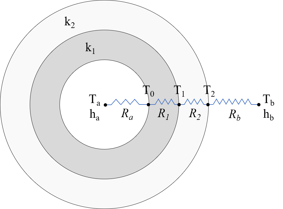
Example 7. A pipe with 5 cm inner diameter and 7.6 cm outer diameter has thermal conductivity k₁= 15 W/mC. It is covered with a 2 cm thick insulation with thermal conductivity k₂= = 0.2 W/mC. A hot gas at T_a = 330 C and h_a = 400 W/m2C flows in the pipe. The outer surface of insulation is exposed to cooler air at T_b = 30 C and h_b = 60 W/m2C.

Calculate heat loss from the pipe to the air if the pipe length is 10 m.

2. Calculate the temperature drop from thermal resistance of the hot gas flow, the pipe material, the insulation, and the outside air.

Ans: i) Heat loss = 7451 W ii) Temperature drop, Ta-T0 = 11.9 C ii) Temperature drop, T0-T1 = 3.3 C ii) Temperature drop, T1-T2 = 250.7 C ii) Temperature drop, T2-Tb = 34.1 C

# Example 7
from pychemengg.heattransfer import steadystate as ss
# Model pipe and insulation each as a Cylinder.
pipe = ss.Cylinder(length=10, inner_radius=0.05/2, outer_radius=0.076/2, thermalconductivity=15)
ins = ss.Cylinder(length=10, inner_radius=0.076/2, outer_radius=0.076/2+0.02, thermalconductivity=0.2)
# The resistances ar as follows:
Ra = pipe.resistanceof_conv(heattransfercoefficient=400, radius=pipe.inner_radius)
R1 = pipe.resistanceof_cond()
R2 = ins.resistanceof_cond()
Rb = ins.resistanceof_conv(heattransfercoefficient=60,radius=ins.outer_radius)
total_R = Ra + R1 + R2 + Rb
total_heatrate = (330-30)/total_R
print(f"Total heat loss = {total_heatrate: .2f} W")
# At steady state heat flow rate is the same for all resistances.
# Temperature drops can therefore be found from deltaT = total_heatrate * Resistance.
delta_Ta_T0 = total_heatrate * Ra
delta_T0_T1 = total_heatrate * R1
delta_T1_T2 = total_heatrate * R2
delta_T2_Tb = total_heatrate * Rb
print(f"Temperature drop, Ta - T0 = {delta_Ta_T0: 0.1f} C")
print(f"Temperature drop, T0 - T1 = {delta_T0_T1: 0.1f} C")
print(f"Temperature drop, T1 - T2 = {delta_T1_T2: 0.1f} C")
print(f"Temperature drop, T2 - Tb = {delta_T2_Tb: 0.1f} C")

# PRINTED OUTPUT
Total heat loss =  7451.73 W
Temperature drop, Ta - T0 =  11.9 C
Temperature drop, T0 - T1 =  3.3 C
Temperature drop, T1 - T2 =  250.7 C
Temperature drop, T2 - Tb =  34.1 C

Example 8: Spherical system `conduction`¶

Example 8. A hollow sphere has inner and outer radii of 4 and 8 cm, respectively. It’s material of construction has a thermal conductivity = 50 W/mC. Find the heat flux needed to maintaint the inner surface at 100 C while the outer surface is at 0 C. Ans: 250 kW/m2

# Example 8
from pychemengg.heattransfer import steadystate as ss
# Model sphere as Sphere.
sphere = ss.Sphere(inner_radius=4e-2, outer_radius=8e-2, thermalconductivity=50)
# Flux = heat rate / surface area
# Here surface area should be inner surface area of sphere.
innerarea = sphere.area(sphere.inner_radius)
heatflux = sphere.heatrateof_cond(dT=100-0)/innerarea
print(f"Heat flux required = {heatflux: e}")

# PRINTED OUTPUT
Heat flux required =  2.500000e+05

====

Example 9: Spherical system `composite shell, conduction, convection`¶

Example 9. A hollow sphere has two layers in perfect thermal contact, an inner layer of lead (k= 35.3 W/mK) and an outer of stainless steel (k=15.1 W/mK). The sphere is filled with radioactive waste, which generates heat at a rate of 5 x 10⁵ W/m3. The outside surface of sphere is exposed to T_infinity = 10 C with heat transfer coefficient of h = 500 W.m2K. The radii of the layers are:

r1 (inner radius of lead layer) = 0.25 m

r2 (outer radius of lead layer) = 0.3 m

r3 (outer radius of stainless steel layer) = 0.31 m

What is the temperature of the innermost layer of the shell at radius r1?

Ans: 405 K

# Example 9
from pychemengg.heattransfer import steadystate as ss
# Model individual layers of shell as Sphere.
layer_lead = ss.Sphere(inner_radius=.25, outer_radius=.30, thermalconductivity=35.3)
layer_SS = ss.Sphere(inner_radius=.30, outer_radius=.31, thermalconductivity=15.1)
# Heat rate can be computed by multiplying volumetric rate of heat generation
# with inner volume of sphere.
heatrate = 5e5 * layer_lead.volume(radius=layer_lead.inner_radius)
# At steady state this is the rate of heat transferred through the shell layers.
# Using heat rate = delta T / resistance, outer temeprature of shell can be found.
total_R = (layer_SS.resistanceof_conv(heattransfercoefficient=500, radius=shellSS.outer_radius)
          + layer_SS.resistanceof_cond()
          + layer_lead.resistanceof_cond())
# delta T = inside temp - 10, form which inside temp can be computed
insidetemp_layer_lead = 10 + heatrate*total_R
print(f"Inside temp of lead shell = {shellLeadTempInside+273: .0f} K")


# PRINTED OUTPUT
Inside temp of lead shell =  405 K

Steady State Heat Transfer¶

Introduction¶

Examples¶

Example 1: Rectangular system conduction¶

Example 2: Rectangular system conduction¶

Example 3: Rectangular system convection¶

Example 4: Rectangular system convection + radiation¶

Example 5: Rectangular system composite wall, conduction¶

Example 6: Cylindrical system convection¶

Example 7: Cylindrical system composite cylinder, conduction, convection¶

Example 8: Spherical system conduction¶

Example 9: Spherical system composite shell, conduction, convection¶